4.2 相关性函数¶

原文	Time Series for Data Science - R Code used in Time Series: A Data Analysis Approach Using R
作者	Guangyu Wei
发布	2025-06-15
状态	Done

1.自相关函数(ACF)¶

\(\text{MA}(q)\)模型¶

为方便起见，将模型写为\(x_t=\sum_{j=0}^q\theta_j w_{t-j}\)，其中\(\theta_0=1\)。因为\(x_t\)是一个白噪声的有限线性组合，所以该过程是平稳地，具有以下自相关函数：

\[\begin{align} \gamma(h) &= \mathrm{cov}(x_{t+h}, x_t) = \mathrm{cov} \left( \sum_{j=0}^{q} \theta_j w_{t+h-j}, \sum_{k=0}^{q} \theta_k w_{t-k} \right) \notag \\\\ &=\begin{cases} \sigma_w^2 \sum_{j=0}^{q-h} \theta_j \theta_{j+h}, & 0 \leq h \leq q \\ 0, & h > q \end{cases}\tag{4.2.1} \end{align} \]

从公式中可以看出。在滞后\(q\)期后的\(\gamma(h)\)处截尾(cut off)是\(\text{MA}(q)\)模型的特征。将式\(\text{4.2.1}\)除以\(\gamma(0)\)得到\(\text{MA}(q)\)的\(\text{ACF}\):

\[\begin{equation}\rho(h) = \begin{cases} \displaystyle\frac{ \sum\limits_{j=0}^{q-h} \theta_j \theta_{j+h} }{ 1 + \theta_1^2 + \cdots + \theta_q^2 }, & 1 \leq h \leq q \\ 0, & h > q \end{cases}\tag{4.2.2} \end{equation} \]

另外我们注意到，因为\(\theta_q\neq0\)，所以\(\rho(q)\neq 0\)。

\(\text{AR}(p)\)和\(\text{ARMA}(p,q)\)模型¶

对于一个\(\text{AR}(p)\)模型或\(\text{ARMA}(p,q)\)模型，将其写为因果\(\text{MA}(\infty)\)的形式：

\[\begin{equation} x_t=\sum_{j=0}^\infty\psi_jw_{t-j} \end{equation}\tag{4.2.3}\]

从而，\(x_t\)的自协方差可以写成

\[\begin{equation} \gamma(h)=\mathrm{cov}\left(x_{t+h},x_{t}\right)=\sigma_{w}^{2}\sum_{j=0}^{\infty}\psi_{j+h}\psi_{j},\quad h\geqslant0\tag{4.2.4} \end{equation}\]

guangyu 注: 动手推推不难得到

\(cov(\sum_{j=0}^\infty\psi_jw_{t-j},\sum_{j=0}^\infty\psi_jw_{t+h-j})=\) \(cov(\psi_0w_t+\psi_1w_{t-1}+...,\psi_0w_{t+h}+\psi_1w_{t+h-1}+...+\psi_hw_t+\psi_{h+1}w_{t-1}+... )\) \(=\sigma_{w}^{2}\sum_{j=0}^{\infty}\psi_{j+h}\psi_{j}\)

ACF由下式给出：

\[\begin{equation} \rho(h)=\frac{\gamma(h)}{\gamma(0)}=\frac{\sum_{j=0}^\infty\psi_{j+h}\psi_j}{\sum_{j=0}^\infty\psi_j^2},\quad h\geqslant0\tag{4.2.5} \end{equation}\]

与\(\text{MA}(q)\)模型不同，\(\text{AR}(p)\)模型和\(\text{ARMA}(p,q)\)模型的\(\text{ACF}\)不在任何滞后期截尾，因此很难使用\(\text{ACF}\)识别\(\text{AR}\)模型或\(\text{ARMA}\)模型的阶数。

2. 偏自相关函数(PACF)¶

在式\(\text{(4.2.2)}\)中，我们看到\(\text{MA}(q)\)的\(\text{ACF}\)值在滞后期大于\(q\)时会变成\(0\)。此外，因为\(\theta_q\neq 0\)，所以\(\text{ACF}\)在滞后期数为\(q\)时并不为\(0\)。因此，当过程是移动平均过程时，\(\text{ACF}\)会提供大量关于依赖性的阶数的信息。

然而，如果过程为\(\text{ARMA}\)或\(\text{AR}\)模型，则单靠\(\text{ACF}\)仅能提供很少关于依赖性的阶数的信息。因此，为了确定\(\text{AR}\)模型的阶数，我们需要找一个像\(\text{MA}(q)\)模型的\(\text{ACF}\)那样可以提供模型阶数信息的函数，这个函数可以为\(\text{AR}\)模型提供阶数信息，称为偏自相关函数。

把上述想法应用到时间序列中，考虑一个因果的\(\text{AR}(1)\)模型\(x_t=\phi x_{t-1}+w_t\)。然后有

\[\begin{aligned}\gamma_{x}(2)&=\operatorname{cov}\left(x_t,x_{t-2}\right)=\operatorname{cov}\left(\phi x_{t-1}+w_t,x_{t-2}\right)\\&=\operatorname{cov}\left(\phi x_{t-1},x_{t-2}\right)=\phi\gamma_x(1)\end{aligned}\]

注意到因果关系中\(cov(w_t,x_{t-2})=0\)，因为\(x_{t-2}\)中含有\({w_{t-2},w_{t-3},...}\)，这些与\(w_t\)不相关。与\(\text{MA}(1)\)一样，\(x_t\)和\(x_{t-2}\)之间的相关性不为\(0\)。因为\(x_t\)通过\(x_{t-1}\)与\(x_{t-2}\)依赖。假设我们通过移除\(x_{t-1}\)来打破这个依赖链。也就是说，我们考虑\(x_t-\phi x_{t-1}\)与\(x_{t-2}-\phi x_{t-1}\)之间的相关性，因为这就是\(x_t\)和\(x_{t-2}\)移除了对\(x_{t-1}\)的依赖性后的相关性，用这样的方式，我们可以打破\(x_t\)和\(x_{t-2}\)之间的依赖链:

\[\begin{equation} \mathrm{cov}\left(x_t-\phi x_{t-1},x_{t-2}-\phi x_{t-1}\right)=\mathrm{cov}\left(w_t,x_{t-2}-\phi x_{t-1}\right)=0 \nonumber \end{equation}\]

我们使用的工具就是偏自相关函数，就是任意\(x_s\)与\(x_t\)去除了两者"中间"的所有线性影响后的相关性。

guangyu 注：

这个地方还不是很清楚，后面解释。

对于\(h=1,2,...\)，一个平稳过程\(x_t\)的 偏自相关函数(PACF) 表示为

\[\begin{equation} \phi_{11}=\mathrm{corr}\left(x_{1},x_{0}\right)=\rho\left(1\right) \end{equation}\]

和

\[\begin{equation} \phi_{hh}=corr\left(x_{h}-\hat{x}_{h},x_{0}-\hat{x}_{0}\right),\quad h\geqslant2 \end{equation}\]

其中 \(\hat{x}_h\) 是 \(x_h\) 对 \(\{x_1, x_2, \cdots, x_{h-1}\}\) 回归得到的结果，\(\hat{x}_0\) 是 \(x_0\) 对 \(\{x_1, x_2, \cdots, x_{h-1}\}\) 回归得到的结果。

因此，由于平稳性，\(\text{PACF}(\phi_{hh})\)是\(x_{t+h}\)和\(x_t\)除去了\(\{x_{t+1},...,x_{t+h-1}\}\)的线性影响后的相关性关系。

\(\text{AR}(p)\)模型¶

对于所有滞后期大于\(p\)的\(\text{AR}(p)\)模型，其\(\text{PACF}\)将为\(0\)，滞后期为\(p\)期的\(\text{PACF}\)不可为\(0\)。因为可以证明\(\phi_{pp}=\phi_{p}\)(模型最后的一个参数)。

对于\(\text{AR}(2)\)模型：

\[\begin{equation} x_t=1.5x_{t-1}-0.75x_{t-2}+w_t \nonumber \end{equation}\]

在这里，\(\phi_{11}=\rho(1)=\phi_1/(1-\phi_2)=1.5/1.75\approx0.86,\phi_{22}=\phi_2=-0.75,\)，对于\(h>2\),\(\phi_{hh}=0\)。

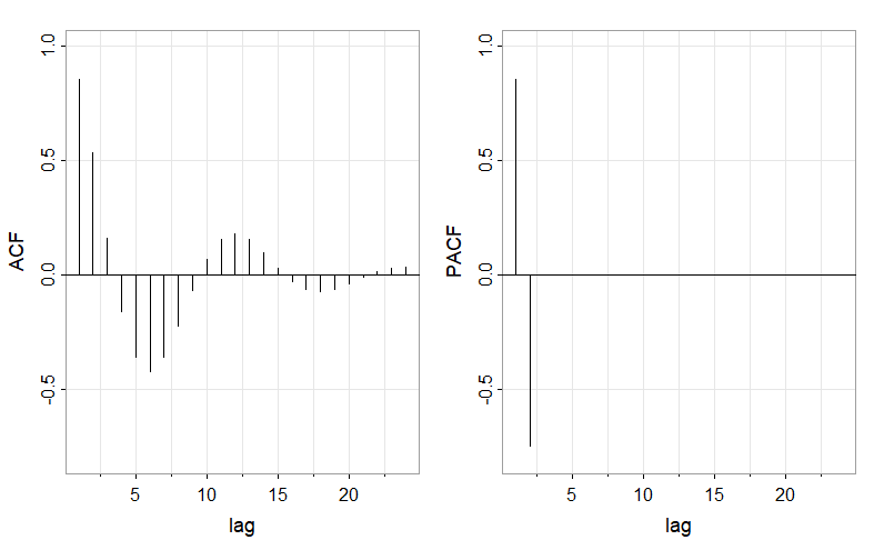
图 4.1：展示了该\(\text{AR}(2)\)模型的\(\text{ACF}\)和\(\text{PACF}\)。

\(\text{MA}(q)\)模型¶

对于可逆的\(\text{MA}(q)\)，具有一个\(\text{AR}(\infty)\):

\[\begin{equation} x_t=-\sum_{j=1}^\infty\pi_jx_{t-j}+w_t \end{equation}\]

此外，模型不存在项数有限的表达式。因此，从这个结果可以明显地看出，该序列的\(\text{PACF}\)不会像\(\text{AR}(p)\)模型一样截尾。对于一个\(\text{MA}(1)\)模型，\(x_t=w_t+\theta w_{t-1}\)，其中\(|\theta|<1\)，可以证明:

\[\begin{equation} \phi_{hh}=-\frac{(-\theta)^h(1-\theta^2)}{1-\theta^{2(h+1)}},\quad h\geqslant1 \end{equation}\]